
Excel Assessment - Businesspersons' Benchmark
Quiz-summary
0 of 15 questions completed
Questions:
- 1
- 2
- 3
- 4
- 5
- 6
- 7
- 8
- 9
- 10
- 11
- 12
- 13
- 14
- 15
Information
Loading test…
You have already completed the quiz before. Hence you can not start it again.
Quiz is loading...
You must sign in or sign up to start the quiz.
You have to finish following quiz, to start this quiz:
Results
Your time:
Time has elapsed
You have reached 0 of 0 points, (0)
| Average score |
|
| Your score |
|
Categories
- B) Businesspersons Benchmark 0%
-
Well done !
Your score is shown above – you need at least 55 points to pass – did you make it??
Next Steps:
1) Click on the “Review your answers…” button below to check our explanations for each question against your answer
2) Take it up a notch and take the next assessment (ready for a challenge?): Excel Advanced Level
3) Return to your dashboard and review answers from there – and download your certificate (Dashboard)

While you are here, can we ask for a favour?
Click here to Challenge a friend! by email
| Pos. | Name | Entered on | Points | Result |
|---|---|---|---|---|
| Table is loading | ||||
| No data available | ||||
- 1
- 2
- 3
- 4
- 5
- 6
- 7
- 8
- 9
- 10
- 11
- 12
- 13
- 14
- 15
- Answered
- Review
-
Question 1 of 15
1. Question
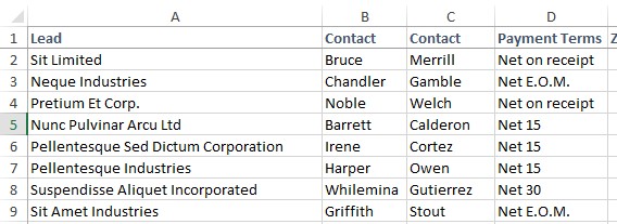
Above is a list with information on customers – complete the missing parts of the VLOOKUP formula below that looks up the Customer Name and shows the Payment Terms as the result of the formula.
- =VLOOKUP(A1,Data! (A:D, $A:$D, A1:D9, $A$1:$D$9), (4), (0, FALSE))
Correct
The first part of this formula is the Lookup value, which was already filled in – A1. This cell contains the Customers Name.
The second part is the Table_array, which in this case refers to the list of information in the image. This is the range address for the list that contains the information you want to look up. To allow for additions to this table, the best options here is to refer to the entire columns – so the formula would like this so far:
=VLOOKUP(A1,Data!A:D,_,_) – by the way – if you entered $A:$D, A1:D9 or $A$1:$D$9 as the answer, this question would still be marked as correct – these are all valid options for this question.
The third setting is the Col_index_num. The VLOOKUP formula looks for the Lookup Value in the first column of the table array. Using our example, the customer name is in cell A1, so it will look for this name in column A, which is the first column of the table array. Once it finds the value it looks for, then uses the Col index number to know what value you want the formula to display. In our example, we wanted to show the customers Payment Terms, which is in column C, which is the 4th column in the table array, so the Col_index_num setting is 4. The formula now looks like this:
=VLOOKUP(A1,Data!A:D,4,_)
The last part of the VLOOKUP formula is just as important as the rest – it’s the Range_Lookup. This needs to be set to 0 or FALSE. It’s important because if it’s left blank, the VLOOKUP will look for the closest match to the value you are looking up, rather than the exact match. In some cases, the closest match is the desired result, but in this case, we want an exact match, so 0 or FALSE is the correct setting here.
The final formula should be: =VLOOKUP(A1,Data!A:D,4,0) or =VLOOKUP(A1,Data!A:D,4,FALSE)
Incorrect
-
Question 2 of 15
2. Question
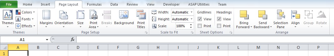
Above is an image of the Ribbon. Caroline has some tasks to do on her sheet – what tabs will she need to go to to complete the following tasks? Assign the tabs to the correct tasks.
Sort elements
- Review Tab
- View Tab
- Data Tab
- Home Tab
- Insert Tab
-
Password protect the sheet
-
Set up the sheet so that when she scrolls the sheet towards to the Right, column A remains visible.
-
Add a drop down list so users can select payment terms from a list
-
Add a special format so that if two or more identical entries are found in the same column, it turns the fill of those cells to red
-
Insert a chart
Correct
Password protect the sheet: This is done on the Review Tab
Set up the sheet so that when she scrolls the sheet towards to the Right, column A remains visible: This is the Freeze Panes function, on the View Tab
Add a drop down list so users can select payment terms from a list: This is done using Data Validation, on the Data Tab
Add a special format so that if two or more identical entries are found in the same column, it turns the fill of those cells to red: This is done using Conditional Formatting, on the Home Tab
Incorrect
Password protect the sheet: This is done on the Review Tab
Set up the sheet so that when she scrolls the sheet towards to the Right, column A remains visible: This is the Freeze Panes function, on the View Tab
Add a drop down list so users can select payment terms from a list: This is done using Data Validation, on the Data Tab
Add a special format so that if two or more identical entries are found in the same column, it turns the fill of those cells to red: This is done using Conditional Formatting, on the Home Tab
-
Question 3 of 15
3. Question
Caroline entered 01/01/2014 in a cell and when she pressed Enter, the value in the cell shows as 41640.00, what does she need to do?
Correct
This is a formatting problem – the cell needs to be formatted as a Date.
Excel stores dates as a number – the number represents the number of days since 1900-Jan-0 – so, the figure that shows up in Caroline’s sheet is a date – 41640 days from 1900-Jan-0 is the 1st of Jan 2014, so all she needs to do is tell Excel to display it as a date as we know them – this is done by formatting the cell as a date.
Incorrect
This is a formatting problem – the cell needs to be formatted as a Date.
Excel stores dates as a number – the number represents the number of days since 1900-Jan-0 – so, the figure that shows up in Caroline’s sheet is a date – 41640 days from 1900-Jan-0 is the 1st of Jan 2014, so all she needs to do is tell Excel to display it as a date as we know them – this is done by formatting the cell as a date.
-
Question 4 of 15
4. Question
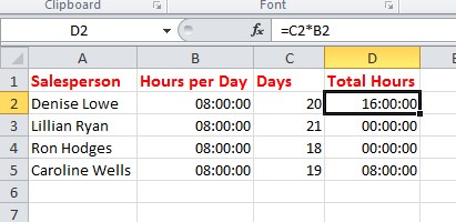
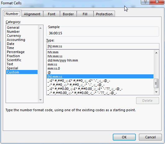
Caroline is calculating total hours worked per employee – she has set up the information above, including a formula in column D that multiplies the hours per day by the amount of days worked, but there is clearly something wrong with this formula. What is the solution?
Correct
The solution to this problem is to format the cell using the [h]:mm:ss format. Excel usually displays time like a 24 hour clock – once it gets to 24 hours, it starts counting again. By formatting it this way, it tells Excel to keep counting on past 24hs.
This is found in the custom list of formats:
 Incorrect
The solution to this problem is to format the cell using the [h]:mm:ss format. Excel usually displays time like a 24 hour clock – once it gets to 24 hours, it starts counting again. By formatting it this way, it tells Excel to keep counting on past 24hs.
This is found in the custom list of formats:
-
Question 5 of 15
5. Question
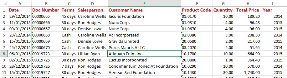
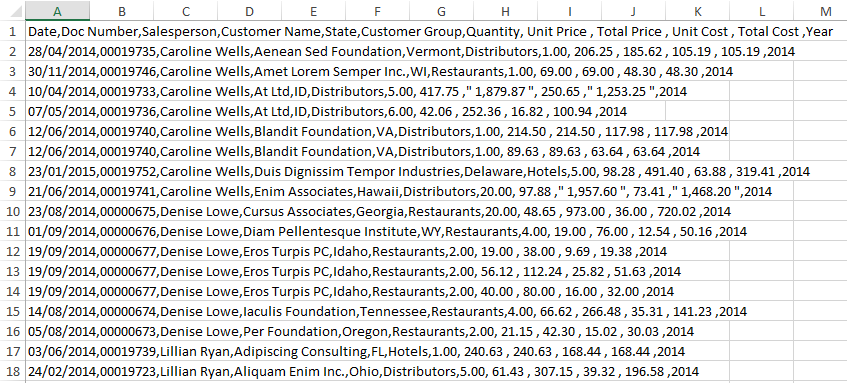
Look at the table of information above – Caroline would like to use a formula to calculate the total of her sales in the year 2014 – which one of the following formulas should she use?
Correct
In this case a simple SUMIF formula will not work because there is more than one criteria to be applied – we need to sum only sales where Caroline is the salesperson, for the year 2014. In this case you can use a SUMIFS formula. The formula for this example would be: =SUMIFS(H:H,I:I,2014,D:D,”Caroline Wells”). Of course you could type Caroline’s name and the year into a cell each, and then refer to the cell addresses rather than the actual values – like this: =SUMIFS(H:H,I:I,A1,D:D,A2) – that would make it easier to change the formulas to look up another persons sales.
Incorrect
In this case a simple SUMIF formula will not work because there is more than one criteria to be applied – we need to sum only sales where Caroline is the salesperson, for the year 2014. In this case you can use a SUMIFS formula. The formula for this example would be: =SUMIFS(H:H,I:I,2014,D:D,”Caroline Wells”). Of course you could type Caroline’s name and the year into a cell each, and then refer to the cell addresses rather than the actual values – like this: =SUMIFS(H:H,I:I,A1,D:D,A2) – that would make it easier to change the formulas to look up another persons sales.
-
Question 6 of 15
6. Question
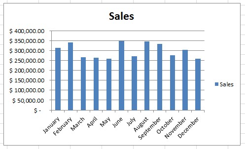
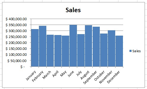
Caroline would like to change the chart shown above so it looks more like this one here:
What does she have to do?
Correct
The answer to this on is she needs to set the gap width for the Data Series to 5%.
You do this by right clicking on one of the bars and selecting Format Data Series. That then gives you the option to set the gap width as a percentage, in this case she used 5%.
Incorrect
The answer to this on is she needs to set the gap width for the Data Series to 5%.
You do this by right clicking on one of the bars and selecting Format Data Series. That then gives you the option to set the gap width as a percentage, in this case she used 5%.
-
Question 7 of 15
7. Question
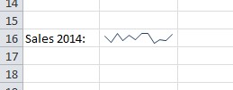
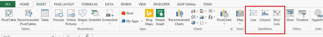
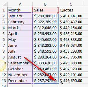
The line chart shown above is not a normal type of chart – enter the name for this type of chart:
- It's a (sparkline, Sparkline, spark line, Spark line) chart.
Correct
This is a Sparkline chart and they are small charts that fit inside a cell. This particular one is a line chart, you can also insert a bar chart or what Excel calls a Win/Loss chart.
To use one, you need to click on the cell where you want it to appear, then go to the Insert Menu and locate the Sparkline charts. Click on the one you want to use, and it will ask you to specify the range of data you want to use. Simply select the data you want to display and then click OK.
 Incorrect
This is a Sparkline chart and they are small charts that fit inside a cell. This particular one is a line chart, you can also insert a bar chart or what Excel calls a Win/Loss chart.
To use one, you need to click on the cell where you want it to appear, then go to the Insert Menu and locate the Sparkline charts. Click on the one you want to use, and it will ask you to specify the range of data you want to use. Simply select the data you want to display and then click OK.
-
Question 8 of 15
8. Question
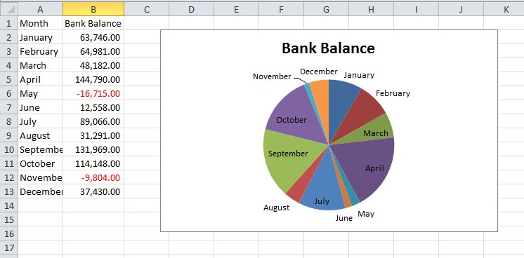
Have a look at the information that has been plotted on the Pie Graph – look carefully at the data used to prepare this Pie Graph – is this graph a true representation of the data?
Correct
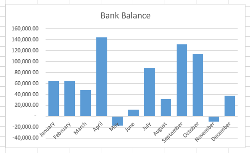
This pie graph is not a true representation of the data because the data includes a negative number which a Pie graph cannot display – in fact it displays it as a positive number.
A better chart to use in this case would be a bar or line graph:
 Incorrect
This pie graph is not a true representation of the data because the data includes a negative number which a Pie graph cannot display – in fact it displays it as a positive number.
A better chart to use in this case would be a bar or line graph:
-
Question 9 of 15
9. Question
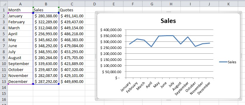
Caroline needs to add the data in column C to this chart – what’s the quickest way of doing this?
Correct
The quickest way to do this is to simply click on the chart, and then drag the selection handles on the data range across to include the extra data.
 Incorrect
The quickest way to do this is to simply click on the chart, and then drag the selection handles on the data range across to include the extra data.
-
Question 10 of 15
10. Question
Caroline has a list with thousands of products and their sell prices. The formula has some confidential information in it that she does not want anyone to see – how does she remove the formulas but leave the values in place?
Correct
To replace formulas with their values, you need to copy the cells that contain the formulas, and then paste over them using Paste Special > Values.
Incorrect
To replace formulas with their values, you need to copy the cells that contain the formulas, and then paste over them using Paste Special > Values.
-
Question 11 of 15
11. Question
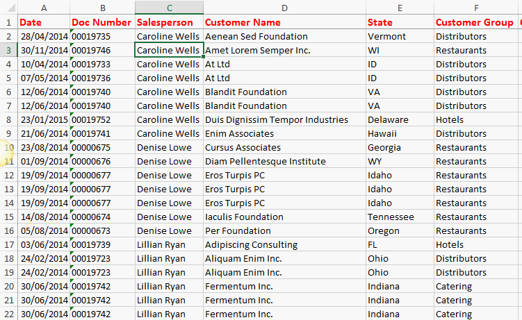
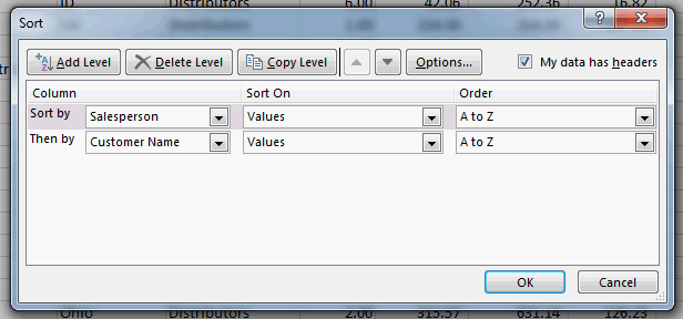
The information above has been sorted by more than one column. Below are images of the Sort dialogue window set up to sort in different ways – which one would sort the data displayed in the image above?
Correct
This information is sorted by Salesperson and then by Customer Name. The correct setting for this is:
 Incorrect
This information is sorted by Salesperson and then by Customer Name. The correct setting for this is:
-
Question 12 of 15
12. Question
Caroline has downloaded a report from their accounting system and it looks like the image above. What tool will she need to use to get this into proper tabular format?
Correct
She needs to use the Text to Columns tool.
 Incorrect
She needs to use the Text to Columns tool.
-
Question 13 of 15
13. Question
Caroline has created this formula in a cell: =(20*5)/(15*5).
Why has she used parenthesis in this formula?
Correct 5 / 5PointsThe use of parenthesis tells Excel in what order the different calculations need to be calculated. This happens in maths as well.
Excel calculates the multiplication and division parts of a formula first, and then the addition and subtraction parts.
The result of the formula above is 1.33 when used this way, and 33.33 when used without parenthesis. And here’s why:
With the parenthesis, the formula first calculates the amounts in parenthesis, so the calculation Excel does is actually =100/75, which is 1.33
Without the parenthesis, the formula Excel multiplies 15 by 5, which is 75, and then divides 5 by 75 – which gives us 1.67. Lastly it multiplies this amount by 20 – giving us 33.33
Incorrect / 5 PointsThe use of parenthesis tells Excel in what order the different calculations need to be calculated. This happens in maths as well.
Excel calculates the multiplication and division parts of a formula first, and then the addition and subtraction parts.
The result of the formula above is 1.33 when used this way, and 33.33 when used without parenthesis. And here’s why:
With the parenthesis, the formula first calculates the amounts in parenthesis, so the calculation Excel does is actually =100/75, which is 1.33
Without the parenthesis, the formula Excel multiplies 15 by 5, which is 75, and then divides 5 by 75 – which gives us 1.67. Lastly it multiplies this amount by 20 – giving us 33.33
-
Question 14 of 15
14. Question
Caroline has set up this IF formula:
=IF(A1<10,”Below Target”,10*5)
Please explain what the result of this formula will be by filling in the missing words below.
- If the value in cell (A1) is (less, smaller) than 10, then the result of the formula will be " (Below Target)", otherwise, the result will be (50).
Correct
The result of this formula depends on the value in cell A1. If the value in cell A1 is less than 10, then the result of the formula will be “Below Target”, otherwise, the result will be 50.
The IF is a conditional formula, which means it has three parts to it – a condition which will either be TRUE or FALSE – in this example, the condition is “A1<10” – which means in words means “Is the value in cell A1 less than 10” – this will either be True or False.
The next part of the formula is what the formula should show is the condition is True – in this example, it will show “Belo Target. The last part is what to show if the condition is False – and in the example we used a simple formula – 10*5, so the result of the formula will be 50 if the value of A1 is over 10.
Incorrect
The result of this formula depends on the value in cell A1. If the value in cell A1 is less than 10, then the result of the formula will be “Below Target”, otherwise, the result will be 50.
The IF is a conditional formula, which means it has three parts to it – a condition which will either be TRUE or FALSE – in this example, the condition is “A1<10” – which means in words means “Is the value in cell A1 less than 10” – this will either be True or False.
The next part of the formula is what the formula should show is the condition is True – in this example, it will show “Belo Target. The last part is what to show if the condition is False – and in the example we used a simple formula – 10*5, so the result of the formula will be 50 if the value of A1 is over 10.
-
Question 15 of 15
15. Question
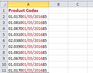
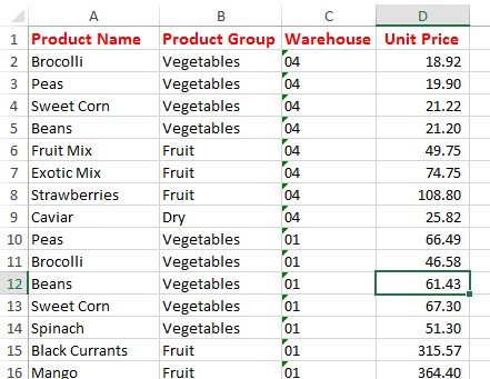
Above is a list of product codes made up of three parts – the first 7 digits is the actual product code, for example, 01.0170. The second part in red is the expiry date – for example, 01/05/2016, and the last two digits is the warehouse number.
Caroline needs a formula in column B that will show just the expiry date – below is the formula that she needs to use – complete the missing parts.
- = (MID)(A2, (8), (10))
Correct
The correct settings for this formula are: =MID(A2,8,10).
The MID formula allows you to extract a portion of text out of a larger text string.
To explain the formula in this example, A2 is the cell which contains the text. 8 is the starting point of the portion of text you want to extract, and 10 is how many characters you want to extract.
If you refer back to the image above, the first part of the date is the 8th character in the text, and the date has 10 characters, so the formula is =MID(A2,8,10)
Incorrect
The correct settings for this formula are: =MID(A2,8,10).
The MID formula allows you to extract a portion of text out of a larger text string.
To explain the formula in this example, A2 is the cell which contains the text. 8 is the starting point of the portion of text you want to extract, and 10 is how many characters you want to extract.
If you refer back to the image above, the first part of the date is the 8th character in the text, and the date has 10 characters, so the formula is =MID(A2,8,10)
Lost your password?