
Excel Assessment - The Fundamentals
Quiz-summary
0 of 15 questions completed
Questions:
- 1
- 2
- 3
- 4
- 5
- 6
- 7
- 8
- 9
- 10
- 11
- 12
- 13
- 14
- 15
Information
Loading test…..
You have already completed the quiz before. Hence you can not start it again.
Quiz is loading...
You must sign in or sign up to start the quiz.
You have to finish following quiz, to start this quiz:
Results
Your time:
Time has elapsed
You have reached 0 of 0 points, (0)
| Average score |
|
| Your score |
|
Categories
- A) The Fundamentals 0%
-
Well done !
Your score is shown above – you need at least 55 points to pass – did you make it??
Next Steps:
1) Click on the “Review your answers…” button below to check our explanations for each question against your answer
2) Take it up a notch and take the next assessment: Excel Businesspersons Benchmark
(Note: If you are a business user, your goal should be to pass the Excel Businesspersons Benchmark Assessments as well)
3) Return to your dashboard and review answers from there – and download your certificate (Dashboard)

While you are here, can we ask for a favour?
Click here to Challenge a friend! by email
| Pos. | Name | Entered on | Points | Result |
|---|---|---|---|---|
| Table is loading | ||||
| No data available | ||||
- 1
- 2
- 3
- 4
- 5
- 6
- 7
- 8
- 9
- 10
- 11
- 12
- 13
- 14
- 15
- Answered
- Review
-
Question 1 of 15
1. Question
Below is a simple formula. Enter the missing character at the beginning of the formula.
- (=, +)A1*20
Correct
All formulas should start with an equals sign: =A1*20. You can use also use a + sign, although this isn’t normal practise.
Incorrect
All formulas should start with an equals sign: =A1*20. You can use also use a + sign, although this isn’t normal practise.
-
Question 2 of 15
2. Question
Keyboard shortcuts are a combination of keys you press together to give commands to Excel. Below is the shortcut for saving a workbook – complete the missing key.
- CTRL + (S)
Correct
The key for saving a workbook is CTRL and S. This is a good shortcut to learn immediately as it is a good idea to save your work on a regular basis in case your computer crashes unexpectedly. This allows you to save your work without having to leave the keyboard to use the mouse.
Incorrect
The key for saving a workbook is CTRL and S. This is a good shortcut to learn immediately as it is a good idea to save your work on a regular basis in case your computer crashes unexpectedly. This allows you to save your work without having to leave the keyboard to use the mouse.
-
Question 3 of 15
3. Question
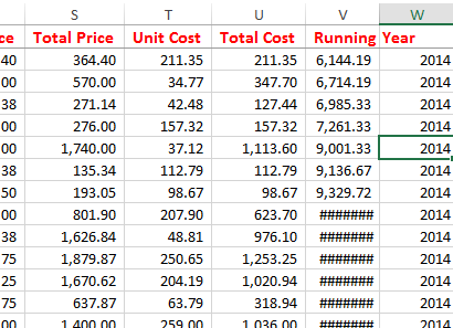
Caroline appears to come across a problem in this sheet. The column V contains a formula that adds up all the sales, keeping a running total. Why are the hashes showing instead of the correct totals?
Correct
The hashes appear when the column isn’t wide enough to display the contents of the cell.
Incorrect
The hashes appear when the column isn’t wide enough to display the contents of the cell.
-
Question 4 of 15
4. Question
Caroline needs to do several tasks on her worksheet – below is the list of things she needs to do – match them up with the ribbon where she would find the tool she needs
Sort elements
- Home Tab
- Insert Tab
- Page Layout Tab
- View Tab
-
Fill the some cells with a blue fill colour
-
Insert an image which contains the company Logo
-
Change the page size to A4
-
Set the Zoom to 100%
Correct
Fill the some cells with a blue fill colour: The cell fill tool is on the Home Tab.
Insert an image which contains the company Logo: The insert picture tool used for this in on the Insert tab.
Change the page size to A4: You would use the Page size setting on the Page Layout tab for this.
Set the Zoom to 100%: The zoom controls are in the View Tab – although it is actually quicker to use the controls in the bottom right hand corner of Excel.
Incorrect
Fill the some cells with a blue fill colour: The cell fill tool is on the Home Tab.
Insert an image which contains the company Logo: The insert picture tool used for this in on the Insert tab.
Change the page size to A4: You would use the Page size setting on the Page Layout tab for this.
Set the Zoom to 100%: The zoom controls are in the View Tab – although it is actually quicker to use the controls in the bottom right hand corner of Excel.
-
Question 5 of 15
5. Question
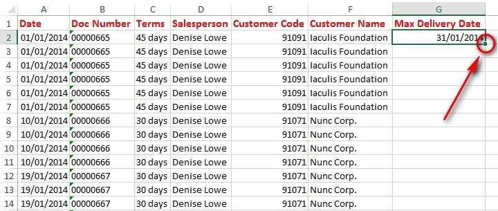
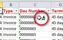
Refer to the image above – the cell fill handle has been circled. You need to fill this formula down the rest of the rows in this workbook – over a thousand cells. Which of the options below would you use to quickly do this?
Correct
The quickest way to copy the contents of a cell to other cells below it is to double click the Fill Handle – you would have scored 5 points if you selected this answer. This only works when there is data in a column next to the column you are working in, and it will only copy down as far as the data in a column next to it.
You can also click and drag the cell handle down – but that is not as quick – you would get 2 points if you chose that option.
Incorrect
The quickest way to copy the contents of a cell to other cells below it is to double click the Fill Handle – you would have scored 5 points if you selected this answer. This only works when there is data in a column next to the column you are working in, and it will only copy down as far as the data in a column next to it.
You can also click and drag the cell handle down – but that is not as quick – you would get 2 points if you chose that option.
-
Question 6 of 15
6. Question
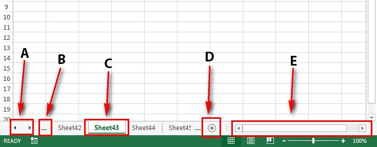
Above is an image of a workbook with dozens of sheets – you need to quickly go to Sheet60. There are several areas outlined – which one do you right click to open a dialogue box where you could quickly jump to Sheet60?
Correct
The answer to this question is A. When you right click this area, a window will open up with a list of all your sheets – you can then quickly move through the list and select the one you want.
Incorrect
The answer to this question is A. When you right click this area, a window will open up with a list of all your sheets – you can then quickly move through the list and select the one you want.
-
Question 7 of 15
7. Question
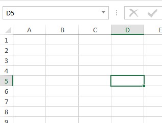
Refer to the image above – which is the address of the selected cell?
Correct
If you know the game “Battleships” you will immediately understand the address of a cell – it is the intersection of the column letter and by the row number. In this case, the activated cell is D5. If you refer to the image above, the address is also displayed in the name box just above cell A1.
Incorrect
If you know the game “Battleships” you will immediately understand the address of a cell – it is the intersection of the column letter and by the row number. In this case, the activated cell is D5. If you refer to the image above, the address is also displayed in the name box just above cell A1.
-
Question 8 of 15
8. Question
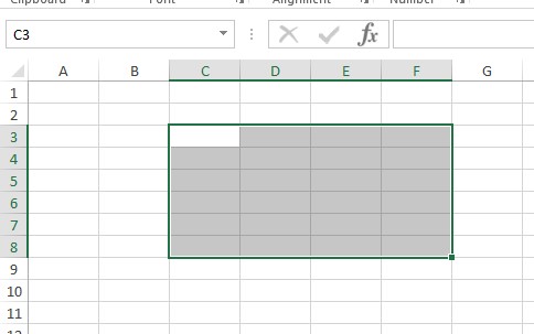
Refer to the image above – a range of cells is selected. What is the address of the selected cells?
Correct
The address of a range of cells is made up of two individual cell addresses – the cell in the top left hand corner, and the cell in the bottom right hand corner. The top addresses are joined with a colon (:) – so the address of the selected cells in this question is C3:F8.
Incorrect
The address of a range of cells is made up of two individual cell addresses – the cell in the top left hand corner, and the cell in the bottom right hand corner. The top addresses are joined with a colon (:) – so the address of the selected cells in this question is C3:F8.
-
Question 9 of 15
9. Question
Caroline has a list of sales for the year, and she would like to see the sales of a particular customer – what tool does she use to hide all the other rows of information, leaving just the rows for the customer she want’s to look at?
Correct
The correct answer is the Filter. By using a filter on your information, you can quickly hide information showing you just the information you want to see. For example if you have a list of sales for the year, you could use a filter to see just the sales of a specific customer without deleting the rest of the information.
Incorrect
The correct answer is the Filter. By using a filter on your information, you can quickly hide information showing you just the information you want to see. For example if you have a list of sales for the year, you could use a filter to see just the sales of a specific customer without deleting the rest of the information.
-
Question 10 of 15
10. Question
Caroline is applying the final touch to the look of her workbook – have a look at the little icon circled above – what tool is she using?
Correct
The tool being used in this image is the Format Painter. It is a quick way of applying formatting you have used on one cell to other cells. Tip: If you need to use the paint brush on many different cells, double click the Format Painter icon and it will stay “active” until you click the icon again, or press the ESC key.
Incorrect
The tool being used in this image is the Format Painter. It is a quick way of applying formatting you have used on one cell to other cells. Tip: If you need to use the paint brush on many different cells, double click the Format Painter icon and it will stay “active” until you click the icon again, or press the ESC key.
-
Question 11 of 15
11. Question
Caroline has selected some cells on this sheet – what is the average of all the selected cells?
Correct
Information on the selected cells is displayed in the status bar at the bottom of the Excel window – information here can show you the sum, count, average and can be configured to show you many other mathematical information. This is a quick way of knowing the sum of a range of cells in your sheet without having to type a formula or use a calculator.
Incorrect
Information on the selected cells is displayed in the status bar at the bottom of the Excel window – information here can show you the sum, count, average and can be configured to show you many other mathematical information. This is a quick way of knowing the sum of a range of cells in your sheet without having to type a formula or use a calculator.
-
Question 12 of 15
12. Question
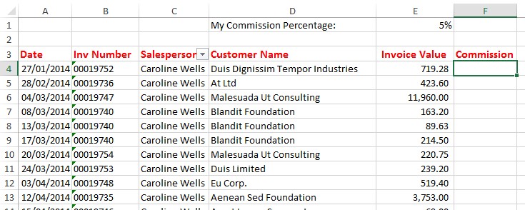
Caroline has got a list of her sales and needs to work out how much her commission is for each sale. Refer to the image above, her commission percentage is in cell E1. She needs a formula that she can enter in cell F4 and copy down the rest of the cells – but beware! The formula needs to always refer to cell E1. Below is part of this formula – complete the missing part.
- =E4* ($E$1, E$1)
Correct
When a formula contains the address of another cell, it normally stores this address as a relative reference – using an example – you can refer to the house next to you as the “house next door” – when you move house, the “house next door” is now a different house – it moves with you, so to speak. Excel formulas work the same way – for example, if you entered this formula as =E4*E1 – when you copy the formula to the cell below, the formula will change to =E4*E2, so it no longer points to the cell that contains the commission.
The solution to this problem is to use an absolute reference – using the example of the house, this would be like it’s address – “107 Kirkbride Road” – no matter where you move, “107 Kirkbride Road” still points to the same house. The way you do this in Excel is use $ signs in the cell address. So the correct answer to this question is =E4*$E$1 or =E4*E$1. When you place a $ before the column letter, this freezes the column, but not the row – which means if you copy the formula to cells on the left or to the right, it will still point to column E, but if you copy the formula down or up rows, the row number will change – so the row number will change, but the column letter will not. The same goes when you place a $ sign in front of the row number. When you use a $ sign on both the column letter and number, the formula will always point to this cell.
The reason the answer could be =E4*$E$1 or =E4*E$1 is because the first option pins the formula to that cell, and the second option pins it to the row – but because in the example the formula was only being copied down, and not sideways, it will still point at the right cell.
We consider this basic knowledge of Excel because without knowing this, errors can be made with even the most basic formulas.
Incorrect
When a formula contains the address of another cell, it normally stores this address as a relative reference – using an example – you can refer to the house next to you as the “house next door” – when you move house, the “house next door” is now a different house – it moves with you, so to speak. Excel formulas work the same way – for example, if you entered this formula as =E4*E1 – when you copy the formula to the cell below, the formula will change to =E4*E2, so it no longer points to the cell that contains the commission.
The solution to this problem is to use an absolute reference – using the example of the house, this would be like it’s address – “107 Kirkbride Road” – no matter where you move, “107 Kirkbride Road” still points to the same house. The way you do this in Excel is use $ signs in the cell address. So the correct answer to this question is =E4*$E$1 or =E4*E$1. When you place a $ before the column letter, this freezes the column, but not the row – which means if you copy the formula to cells on the left or to the right, it will still point to column E, but if you copy the formula down or up rows, the row number will change – so the row number will change, but the column letter will not. The same goes when you place a $ sign in front of the row number. When you use a $ sign on both the column letter and number, the formula will always point to this cell.
The reason the answer could be =E4*$E$1 or =E4*E$1 is because the first option pins the formula to that cell, and the second option pins it to the row – but because in the example the formula was only being copied down, and not sideways, it will still point at the right cell.
We consider this basic knowledge of Excel because without knowing this, errors can be made with even the most basic formulas.
-
Question 13 of 15
13. Question
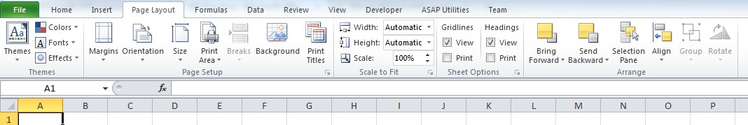
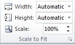
The image above shows the page layout tab. Which group of commands would you use to automatically scale the sheet to fit on one sheet of paper when printed out?
Correct
To make a sheet fit on one page of paper when printed out, you need to set the Width and Height to 1 page on the scale to fit settings:
 Incorrect
To make a sheet fit on one page of paper when printed out, you need to set the Width and Height to 1 page on the scale to fit settings:
-
Question 14 of 15
14. Question
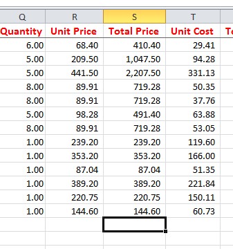
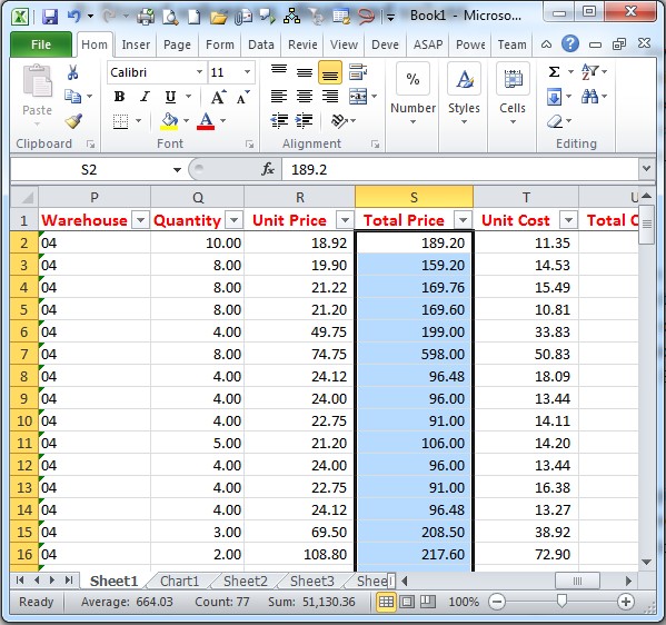
Caroline needs to quickly insert a total amount for the values in the Total Price column – which icon should she click to do this automatically? Select from the options below.
Correct
The icon for autosum is this one:

When you use this tool, it will automatically insert a formula that sums up the values in cells above it. This saves you from having to type a formula.
Incorrect
The icon for autosum is this one:
When you use this tool, it will automatically insert a formula that sums up the values in cells above it. This saves you from having to type a formula.
-
Question 15 of 15
15. Question
Caroline would like to send a sheet to a customer and she doesn’t want the customer to change any of the information on the sheet – select which option she should use:
Correct
The only real safe way to send information to someone without them being able to easily change the contents or see the formulas you have used is to send it as a PDF:
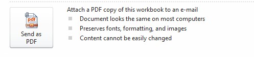
Remember that the formulas you use could give away information you don’t want the customer to see. Also if you have hidden columns, these could be unhid by someone else, revealing information you don’t want them to see – that is not possibly with a PDF.
Incorrect
The only real safe way to send information to someone without them being able to easily change the contents or see the formulas you have used is to send it as a PDF:
Remember that the formulas you use could give away information you don’t want the customer to see. Also if you have hidden columns, these could be unhid by someone else, revealing information you don’t want them to see – that is not possibly with a PDF.
Lost your password?